Thursday, July 31, 2008

Membrane Detection with just simple edge detection

Today, I tried playing around with the membrane data set. I did the following
  1. Created a difference of Gaussian image in GIMP
  2. Enhanced the contrast in GIMP
  3. Thresholded the image in MATLAB
  4. Removed the connected components in the binary image that where less than
    1. Specified Area
    2. Major axis length
  5. The overlay image was created.
The result of such a pipeline is shown below

Wednesday, July 30, 2008

Is there a bug in Invariant Moments?

Today I was inspecting the accuracy of the invariant moments generated by my code and Dr. Tolga's code. I did two different inspections
  1. The moment values from specific points in sample images
  2. Histograms of the moments calculated for sample images
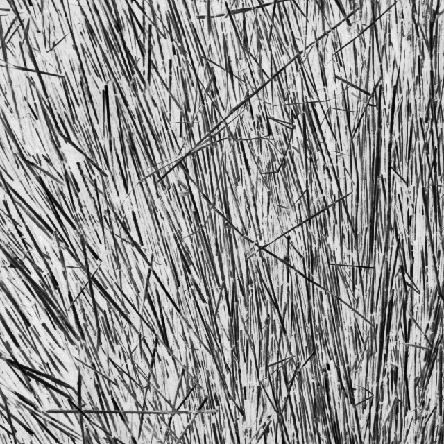
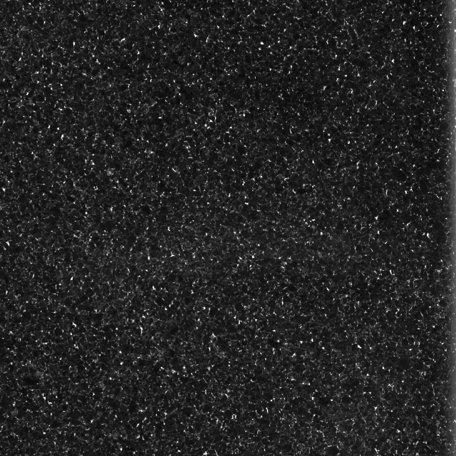
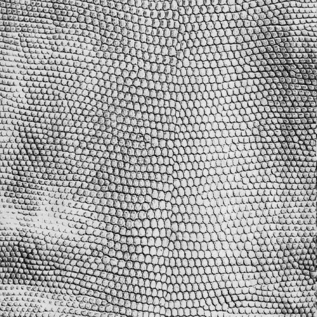
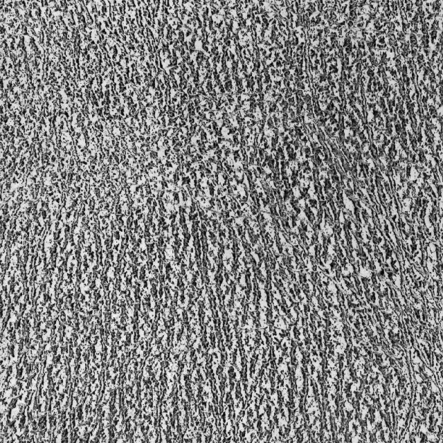
The sample images selected are:


These sample images are 100x100 images.
The moment were calculated values at (50,50) in all the 3 images using my code and Dr. Tolga's code. The results where the following.

For the dots.png image the attributes where compared. The disk sizes taken where 5, 9, 15, 19, 25. The histogram values matched perfectly for both algorithms. Which means they were working on the same circular regions. On comparing the moment values the following where the differences. First row is Dr. Tolga's output and second was mine (For Disk Size 5). The Gram Schmidt operation was also removed from the templates.

1.0e+06 *
0.0066 0.0199 0.0689 0.0689 3.9246 0.2424 -0.0001

0.0000 0.0000 0.0000 0.0000 -0.0000 -0.0000 -0.0000

Updates to this blog can be found in the following blog http://synapseslayer.blogspot.com/2008/07/changing-feature-vector.html

Monday, July 28, 2008

Machine Learning on membrane detection problem

After the reasonable classification of the tougher Brodatz dataset, we move on to a bit tougher problem of membrane detection. There is some ground truth markup of the membranes done by Liz. The dataset can be found in the following location
/usr/sci/crcnsdata/CRCNS/Synapses/data/CellMembraneDetection
The example raw image and the ground truth markup image is shown below


Experiment setup: For this experiment there will be no key point generation. We will iterate through all the pixels in the image and learn over them. The attributes used will be the moments and the histogram bin values for different sized regions. We will be learning using the perceptron based linear classifier and the Decision stump models. The output will also be a image similar to the ground truth image. An overlay image like the one shown below(Ground truth markup over the original) will be created with the predicted membranes.

The feature vectors have been created for the image for all the points on the image with disk Sizes of 5, 10, 15, 20, 25. The feature vector has been stored in the following location.
/usr/sci/crcnsdata/CRCNS/Synapses/data/CellMembraneDetection/
Feature vector: stom-003-regionAttributes-diskSizes-5-10-15-20-25.mat
Y vector: stom-003_clahe_diff_thresh_concomp_thin_edit-yn-25.mat

The attributes look almost inseparable one such attribute is shown in the below figure

Friday, July 25, 2008

Normalizing the invariant moments

Today, I just modified the feature generation code by normalizing the moment generation parameters. Previously for different disk sizes the radii's were taken as is and moments where calculated. So if the disk size is say 30 pixels then the 15^4 would just explode. So in the modified code the radii are normalized to 1.

Brodatz dataset: After this modification the result was run on the tougher Brodatz textures. The following where the results for target prediction rate = 0.8


Synapses dataset: The same experiment on the dataset didn't give any better results. Compared to the previous experiments without fix to the normalization to the moment attributes.

Thursday, July 24, 2008

Fitting in the Linear Classifier

Today, I fitted in the linear classifier code into the cascade architecture. The weak classifier that gets boosted in the nodes is a Perceptron instead of a Decision Stump. The source code can be found in the following directory.
/usr/sci/crcnsdata/CRCNS/Synapses/Code/Matlab/ML_Boosting4_Lin1/

The results of the experiments run on various datasets are shown below.

10D Gaussian dataset: The classifier was able to achieve 100% accuracy (with 0.99 true positive target) with linear classifier.
Brodatz dataset: The classifier was able to achieve 0.9 true positive target in few of the nodes. Here we observe that even though the training examples are the same for nodes 1 & 2 and nodes 6 & 7, they have different performance because the perceptron weight initialization is random in different times.
Synapses dataset: This experiment failed several times because the weak classifier failed to achieve even 50% accuracy. I think this because of the randomization in the weight vectors and the data points used for training. I trained one node once and failed to construct the consecutive nodes. Hence there is no graph for it.

The predicted Y values of every node classifier was giving just 5 or 6 unique values. It has to be more continuous since the sample set is really large. So in the next experiment the moment values where removed from the dataset and the experiment was conducted with a very low true positive rate of 0.7 and the following graphs shows the result of such an approach.


The next step will be verify the moments again and normalize the values. Before starting to work on any other attribute.

Wednesday, July 23, 2008

Fixing the Bug in Threshold Variation

In yesterday's experiment results, we noted that the prediction rate dropping below the required prediction rates even though the minimum prediction rate is set to 0.95 even though the threshold is varied accordingly. This works properly for only few cases and fails in others. The below figure shows a result where the training worked properly with threshold variation at the node.

I did some code changes, and the bug disappeared. After trying a series of experiments, each node of the classifier was able to achieve the desired true positive rate. There were few instances where the classifier went amok. The graph below shows the performance of the classifier at one of these bad instances.


Analyzing why there is sudden increase in the false positive rate, the following was observed in these type of failures. The histogram of output of the boosted classifier (at a particular node) is shown below. The three histograms shows the following:
  1. Blue: Entire distribution of PredictedY [760 0 .. 0 99 14 0 .. 0 727]
  2. Green: Distribution of PredictedY at Y = 1 [ .. 0 0 0 26 5 0 .. 0 727]
  3. Red: Distribution of PredictedY at Y = 0 [760 0 .. 0 73 9 0 .. 0 0]
Here we see that the threshold changing logarithm is not able to find a suitable threshold to achieve the required true positive rate because we change the threshold only to different values of predicted Y (i.e. 0, 3.3620, 3.5603, 6.9223) and not any intermediate values. Here the classifier would have achieve its true positive target if has tried a threshold of say 2.00


The Fix for the above bug was done this way. (Note:The values are different from above since it is a different experiment). For uniqueSortedPredictedY = 0, 3.1102, 3.6728, 6.7830. Intermediate values were also chosen. intermediateValuesOfPredY = 1.5551, 3.3915, 5.2279. This was the also included in the list of possible thresholds and the required true positive rate was achieved for the classifier. I guess this has closed bugs in the Threshold Variation algorithm. Next we will move ahead with the Linear classifier implementation. All the experiments where run on the 10D Gaussian dataset.

Brodatz dataset: After this bug fix, the experiment was run on a the tough Brodatz pattern distinguishing dataset. Since the feature values where finding it difficult to classify at the such high true positive rates the training failed in the first node it self. The distribution of the PredictedY at a node is shown below. A lower target was set and the classifier started to build but failed to move beyond the the 2nd node.
Synapse dataset: The code run for Synapse dataset gave the following training & test results. The true positive target was set at 0.9.
The bug fixed code can be found in /usr/sci/crcnsdata/CRCNS/Synapses/Code/Matlab/ML_Boosting4_DT3 directory. The Boost.m was modified.

Monday, July 21, 2008

Verifying the Feature Vectors

Experiment 1: To verify if the attributes would classify any easy pattern examples the following experiment was conducted.
  1. Two Brodatz textures where chosen.
    1. http://www.ux.uis.no/~tranden/brodatz/D15.gif
    2. http://www.ux.uis.no/~tranden/brodatz/D32.gif
  2. Random points were chosen inside the image. The following code was used to generate the points inside the image. /usr/sci/crcnsdata/CRCNS/Synapses/Code/Matlab/20080721/getPointsFromTexture.m
  3. The features explained in this blog where generated using the code following code. /usr/sci/crcnsdata/CRCNS/Synapses/Code/Matlab/20080721/momentCalc.m. The features are the same. The only difference is that in that experiment the features were generated for SIFT key points where as here it is for random points.
  4. Then the classifier was run over the dataset. The results are as follows.
Experiment 2: The same experiment was run for a different set of images. The features where finding it difficult to segregate these data points into appropriate classes. The images used for this experiment are
  1. http://www.ux.uis.no/~tranden/brodatz/D3.gif
  2. http://www.ux.uis.no/~tranden/brodatz/D24.gif
The classifier would not classify the images correctly. The distribution of the attributes used in the stumps in few of the nodes are noted below. The histograms of different attributes are shown as below:
  1. The blue gives the distribution of the particular attribute for the given data points at that node.
  2. The green histogram is the distribution of the positive synapse regions alone.
  3. The red histogram is the distribution of the negative synapse regions alone.


The below graphs are the different metrics of the classifier that is learned, These are results of one of the successful runs where all 8 nodes of the cascade where constructed. But in most other runs the classifier failed.
The next step is to modify the experiment to fit in the linear classifier instead of the Decision stump classifier.

Verifying the Cascade Classifier

Thursday & Friday, I have been concentrating on verification of the Cascade Machine learning algorithm and the features used in the images.

Verification of Algorithm: To verify the algorithm a simpler dataset was used. It was just a 10D Gaussian dataset with 1000 positive examples and 10,000 negative examples. Generation of 10D dataset was relatively easier using the following MATLAB commands.

posx = 0.25 * randn (10, 1000) + 1; negx = 0.25 * randn (10, 10000) + 0; x = [posx negx]; x = x'; posy = ones (1000,1); negy = ones (10000,1); y = [posy;negy];
The dataset has:
  1. Standard Deviation = 0.25 and mean = 1 for positive examples
  2. Standard Deviation = 0.25 and mean = 0 for negative examples
The figure below shows a 2D dataset with same distribution parameters.
The figure below shows a 2D dataset with distribution parameters S.D. = 0.5 and mean = 0, 1.
The 10D Gaussian dataset was feed to the classifier and the classification results are as shown below.

The machine learning algorithm's classification results for 10D Gaussian dataset are shown in the plots below.


The target prediction rate (true positives) was set at 0.95.

Apart from this, the explanation for very low false positive rate in Dr.Tolga's linear classifier based cascade setup could be the following:
  1. Decision Stump based classifier works on a single attribute at a time the classifying hyperplane is always parallel to the axis of some dimension at anytime whereas for the linear classifier it can find a better classification hyperplane at arbitrary angles to each of the dimensions.
  2. Dr. Tolga's dataset had randomly picked non-synapses locations which could be well inside the lighter regions of the neurons, where as the dataset are confined to darker regions on the image hence making it challenging for the classifier and hence the high false positive rate.

Wednesday, July 16, 2008

The new dataset

Yesterday, the new data set was posted by the Biology team. The new dataset has been placed in the following location
/usr/sci/crcnsdata/CRCNS/Synapses/data/Refined2_marked_RM2_with_fake/

The salient features of the new dataset are:
  • Image is vertical cross section of rabbit retina. The image dimensions are is 11477 x 18361 (Width x Height) .
  • The markup contains synapses arrows where there are synapses (with 100% confidence) and there are few black pin markups that are non-synapses regions but might be misclassified as Synapses. The number of markups are shown below. The number of markups is quite less than the markups in the previous dataset.
    • Synapses - 67
    • Non-synapses - 16
    • Total Markups - 83
Mosaic Builder: Yesterday, I learnt about the usage of Mosaic Builder from a ROI markup perspective alone. I was able to successfully able to install & run Mosaic Builder on pollux.sci.utah.edu in Visualization Lab. Tried out few things like playing with key words of the markups (Marked all the points as Fake!!), exporting the markups so that my MATLAB & QT code could read it.

SynapsesViewer: I fixed a bug in SynapsesViewer where I had hard coded for the positions of the Markups height of the image so that I can view the synapses in my laptop. I shall explain about the SynapsesViewer in a future post.

Tuesday, July 15, 2008

Fixing the bug in the Feature Vector generation for SIFT key points

This is a continuation of the previous blog. This section explains the change in the momentCalc6 function

Bug & Fix: The calculation of the circular regions around the point was done incorrectly. This problem was due to the MATLAB image representation. MATLAB stores top left as (0, 0) where the synapses markup takes the bottom left as the image origin (0,0). To over come this the original image is just flipped upside down so that the region is grabbed correctly. The new data set is stored in the following location:
/usr/sci/crcnsdata/CRCNS/Synapses/data/roiExport3/
The data file names are:
Layer1_0_0_card_resize_p25-nearestSynapseDistance-diskSizes15-30-60-90-120.mat
Layer1_0_0_card_resize_p25-regionAttributes-diskSizes15-30-60-90-120.mat
Layer1_0_0_card_resize_p25-keyPoints-diskSizes15-30-60-90-120.mat
The key points data format has also be changed so as to include the scale and the orientation data from the SIFT data set along with the x, y location of the key points.

After fixing this the learning was done using the Decision Stump based Cascade Classifier. Below is are graphs of the training of the cascade classifier. In the below run, the dataset is skewed ie. Negative examples taken are twice the number of positive examples.


In the next 4 runs, the dataset used is a balanced one. having equal number of positive and negative examples. The positive examples and negative examples get washed out of that particular node as non-synapses, thus after 3 or 4 nodes the cascade runs out of examples to train. I think there is a bug in the DT classifier code with the inequality decision.